American Options and Finite Difference Method
Purpose
We consider an American put option with strike price $K$ and maturity $T$ under the Black-Scholes framework. The underlying asset price $S_t$ is assumed to follow a geometric Brownian motion under the risk-neutral measure $\mathbb{Q}$, described by the stochastic differential equation:
\[dS_t = r S_t dt + \sigma S_t dW_t\]where $r$ is the risk-free interest rate, $\sigma$ is the volatility, and $W_t$ is a standard Brownian motion under $\mathbb{Q}$.
Our objective is to compute the value of the American put option and determine the early exercise boundary using the Finite Difference Method (FDM).
Setup
The Finite Difference Method is a numerical technique for solving partial differential equations (PDEs). It works by discretizing both time and space, converting the continuous PDE into a system of algebraic equations. These equations can then be solved iteratively or directly to approximate the option value at each node of the discretized grid.
In the context of option pricing, FDM enables us to simulate the backward evolution of the option price over time, incorporating the early exercise feature inherent to American options by enforcing the free boundary condition at each time step.
The Obstacle PDE we work on reads as follows
\[\begin{align*} \min \{ \frac{\partial u(x,\tau)}{\partial \tau} - \frac{\partial u(x,\tau)}{\partial x}\,(r-\delta)x-\frac{1}{2}\frac{\partial^2 u(x,\tau)}{\partial x^2} \sigma^2 x^2+ru(x,\tau), \\ \qquad u(x,\tau)-(K-x)_+ \} = 0, \quad\forall \tau (0,T], x\geq0 \end{align*}\]where $\tau = T-t$ is the time to maturity.
The Mesh
We use an implicit scheme, so that the continuation PDE (first term of Obstacle PDE) reads as
\[\frac{u_i^{n+1} - u_i^n}{\Delta t} - \frac{u_{i+1}^{n+1} - u_i^{n+1}}{\Delta x}(r-\delta) x_i - \frac{1}{2}\frac{u_{i-1}^{n+1} - 2u_{i}^{n+1} + u_{i+1}^{n+1}}{(\Delta x)^2} \sigma^2 x_i^2 + ru_i^{n+1} = 0\]Even though this scheme has only first-order precision, it is unconditionally monotone, thus its solution converges locally uniformly to the unique solution of the PDE (Barles-Souganidis Theorem).
\[\begin{align*} u_i^n & = u_{i-1}^{n+1} \underbrace{\left(-\frac{1}{2} \frac{\Delta t}{(\Delta x)^2} \sigma^2 x_i^2 \right)}_{a_i} + u_{i}^{n+1} \underbrace{\left(1+\frac{\Delta t}{\Delta x} (r-\delta)x_i + \frac{\Delta t}{(\Delta x)^2}\sigma^2 x_i^2 + r \Delta t \right)}_{b_i}\\ & \qquad + u_{i+1}^{n+1}\underbrace{\left(-\frac{\Delta t}{\Delta x}(r-\delta) x_i - \frac{1}{2} \frac{\Delta t}{(\Delta x)^2} \sigma^2 x_i^2\right)}_{c_i} \end{align*}\]When written in matrix form we have
\[A_h\mathbf{u}_h^{n+1} = \mathbf{u}_h^n\]where
\[\mathbf{u}_h^n = \begin{bmatrix} \vdots \\ u_{i-1}^n \\ u_i^n \\ u_{i+1}^n \\ \vdots \end{bmatrix}, \quad A_h = \begin{bmatrix} b_0 & c_0 & & & \\ \cdot & \cdot & \cdot & & \\ & \cdot & \cdot & \cdot & \\ & a_i & b_i & c_i & \\ & & \cdot & \cdot & \cdot \\ & & & a_M & b_M \end{bmatrix}.\]So we create a uniform mesh of $M+1$ points in price space and $N+1$ in time space.
Boundary Conditions
We still have to define $b_0, c_0, a_M, b_M$ depending on the boundary conditions we impose on the discretization. The underlying price space will be discretized on a domain $[0,x_{top}]$, where $x_{top}$ is the underlying price after a move of 3 standard deviations:
\[x_{top} = S_0 \exp\{(r-\tfrac{1}{2}\sigma^2)T + 3\sigma \sqrt{T}\}.\]We know that $u(\tau, 0) = K$, and $u(\tau, x_{top}) \sim 0, \forall \tau$, so the vector $\mathbf{u}_h^n$ looks like
\[\mathbf{u}_h^n = [K, \dots, u_{i-1}^n, u_i^{n}, u_{i+1}^n, \dots, 0]^\top,\]So, $b_0 = 1, c_0 = 0, a_M = 0, b_M = 0$.
Inverse of Martrix A
The Thomas algorithm is a simplified form of Gaussian elimination that efficiently solves linear systems where the coefficient matrix is tridiagonal — that is, a matrix where only the main diagonal and the two diagonals directly above and below it are non-zero.
Given a linear system: \(Ax = b\) where $A$ is a triagonal matrix.
The algorithm proceeds in two steps:
- Forward elimination – transform to upper triangular.
- Backward substitution – solve for $x$.
Results
Using $r=0.01, \delta = 0, \sigma = 0.2, K=100, T=1, S_0 = 100 $, we obtain the following results.
Price of American Put Option: 11.4526
Analysis
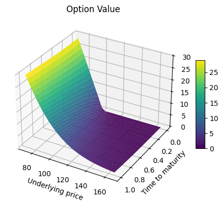
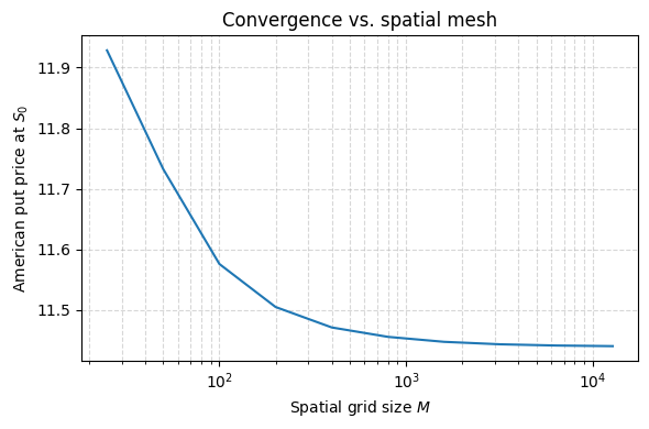
The implicit scheme demonstrates monotonic convergence toward a stable value, as theoretically expected. From the option value surface, we observe how the function deforms near the singularity at the point $(0, K)$. This behavior aligns with known results: solutions to obstacle problems—often formulated as variational inequalities—tend to lack smoothness and may even be discontinuous at certain points. However, in this case, we do not observe additional visible singularities, such as along the free boundary, from visual inspection alone.
The code
import numpy as np
import matplotlib.pyplot as plt
class FDM:
def __init__(self,
r: float,
delta: float,
sigma: float,
K: float,
T: float,
S0: float,
M: int,
N: int,
opt_type: chr):
self.r, self.delta, self.sigma = r, delta, sigma
self.K, self.T, self.S0 = K, T, S0
self.M, self.N = M, N
self.opt_type = opt_type
# time & space steps
self.delta_t = T / N
self.x_top = S0 * np.exp((r - delta - 0.5*sigma**2)*T + 3*sigma*np.sqrt(T))
self.delta_x = self.x_top / M
# grid & payoff
self.time = np.linspace(0, T, N)
self.x = np.linspace(0, self.x_top, M)
if (self.opt_type == 'P'):
self.payoff = np.maximum(K - self.x, 0)
else:
self.payoff = np.maximum(self.x - K, 0)
self.u = self.payoff.copy() # initial condition at t = T
# precompute diagonals
self.a_vec = self._a() # length M-1
self.b_vec = self._b() # length M
self.c_vec = self._c() # length M-1
# decision Boundary
self.free_bound = np.zeros((N,M))
def _a(self):
a = -0.5 * self.delta_t / self.delta_x**2 \
* self.sigma**2 * self.x[1:]**2
a[-1] = 0.0
return a
def _b(self):
b = 1.0 \
+ self.delta_t / self.delta_x * (self.r - self.delta) * self.x \
+ self.delta_t / self.delta_x**2 * self.sigma**2 * self.x**2 \
+ self.r * self.delta_t
b[0] = 1.0
b[-1] = 1.0
return b
def _c(self):
c = - self.delta_t / self.delta_x * (self.r - self.delta) * self.x[:-1] \
- 0.5 * self.delta_t / self.delta_x**2 * self.sigma**2 * self.x[:-1]**2
c[0] = 0.0
return c
def _thomas(self, a, b, c, d):
"""
Solve tridiagonal system A x = d with:
a = sub‑diag (len M-1), b = main‑diag (len M), c = sup‑diag (len M-1)
d = RHS (len M)
Returns x (len M).
"""
M = len(b)
# make copies so we don't overwrite originals
bp = b.copy()
dp = d.copy()
cp = c.copy()
# forward elimination
for i in range(1, M):
w = a[i-1] / bp[i-1]
bp[i] = bp[i] - w * cp[i-1]
dp[i] = dp[i] - w * dp[i-1]
# back substitution
x = np.zeros_like(d)
x[-1] = dp[-1] / bp[-1]
for i in range(M-2, -1, -1):
x[i] = (dp[i] - cp[i] * x[i+1]) / bp[i]
return x
def run(self, early_exercise: bool = True):
"""
Backward using Thomas solver on each step.
"""
for _ in range(self.N-1):
self.u = self._thomas(self.a_vec, self.b_vec, self.c_vec, self.u)
if early_exercise:
# mask = where payoff >= continuation -> we exercise
mask = self.payoff >= self.u
# record free boundary at this time‐step
self.free_bound[_, mask] = 1
# update u: exercise vs continue
self.u = np.where(mask, self.payoff, self.u)
self.free_bound[:,-1] = 0
return self.u
def get_price(self):
return np.interp(self.S0, self.x, self.u)
def get_free_bound(self):
return self.free_bound
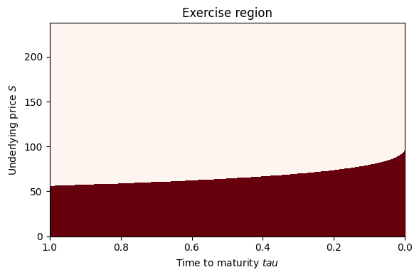
def plot_free_bound(self):
"""
Plot the exercise region as a heatmap.
X–axis: underlying price (self.x)
Y–axis: time (self.time)
free_bound[t,i] == 1 ⇒ exercise
"""
# make a meshgrid for plotting
T, X = np.meshgrid(self.time, self.x, indexing='ij')
plt.figure(figsize=(6,4))
plt.pcolormesh(
T, X,
self.free_bound,
shading='auto',
cmap='Reds'
)
plt.xlabel('Time to maturity $tau$')
plt.ylabel('Underlying price $S$')
plt.title('Exercise region')
plt.gca().invert_xaxis()
plt.tight_layout()
plt.show()
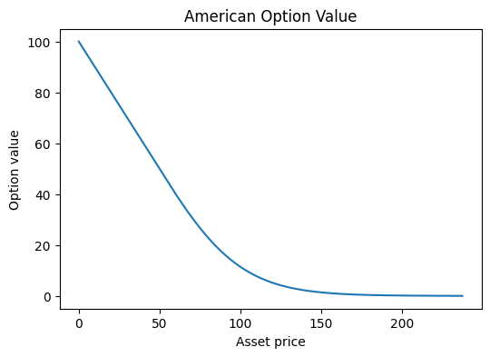
def plot_value(self):
plt.figure(figsize=(6,4))
plt.plot(self.x, self.u)
plt.xlabel('Asset price')
plt.ylabel('Option value')
plt.title('American Option Value')
plt.show()
def plot_value_surface(self, early_exercise: bool = True):
X, Y = np.meshgrid(self.x[int(self.M*0.3):int(self.M*0.7)], self.time)
u = np.zeros((self.N, self.M))
u[0,:] = self.payoff.copy()
for i in range(self.N-1):
u[i+1,:] = self._thomas(self.a_vec, self.b_vec, self.c_vec, u[i,:])
if early_exercise:
u[i+1,:] = np.maximum(u[i+1,:],self.payoff)
fig = plt.figure(figsize=(6, 4))
ax = fig.add_subplot(111, projection='3d')
surf = ax.plot_surface(X, Y, u[:,int(self.M*0.3):int(self.M*0.7)],
cmap='viridis', edgecolor='none')
# 4. Add labels and color bar
ax.set_title('Option Value')
ax.set_xlabel('Underlying price')
ax.set_ylabel('Time to maturity')
fig.colorbar(surf, shrink=0.5, aspect=10)
plt.gca().invert_yaxis()
plt.tight_layout()
plt.show()
r=0.01
delta = 0.0
sigma=0.3
K=100
T=1.0
S0=100

solver = FDM(r=r,
             delta=delta,
             sigma=sigma,
             K=K,
             T=T,
             S0=S0,
             M=1000,
             N=1000,
             opt_type='P')

solver.run(early_exercise=True)
solver.plot_value()
solver.plot_free_bound()
print(f"Price of American Put Option: {solver.get_price():.4f}")
solver.plot_value_surface()
M_list = [25, 50, 100, 200, 400, 800, 1600, 3200, 6400, 12800]
prices = []
for M in M_list:
    solver = FDM(r=r, delta=delta, sigma=sigma, K=K, T=T, S0=S0,
            M=M,
            N=1000,
            opt_type='P')

    solver.run(early_exercise=True)
    prices.append(solver.get_price())

plt.figure(figsize=(6,4))
plt.plot(M_list, prices)
plt.xscale('log')
plt.xlabel('Spatial grid size $M$')
plt.ylabel('American put price at $S_0$')
plt.title('Convergence vs. spatial mesh')
plt.grid(True, which='both', ls='--', alpha=0.5)
plt.tight_layout()
plt.show()